S2 Cells
The S2 library defines a framework for decomposing the unit sphere into a hierarchy of cells. Each cell is a quadrilateral bounded by four geodesics. The top level of the hierarchy is obtained by projecting the six faces of a cube onto the unit sphere, and lower levels are obtained by subdividing each cell into four children recursively. For example, the following image shows two of the six face cells, one of which has been subdivided several times:
Notice that the cell edges appear to be curved; this is because they are spherical geodesics, i.e., straight lines on the sphere (similar to the routes that airplanes fly).
Each cell in the hierarchy has a level, defined as the number of times the cell has been subdivided (starting with a face cell). Cells levels range from 0 to 30. The smallest cells at level 30 are called leaf cells; there are 6 * 430 of them in total, each about 1cm across on the Earth’s surface. (Details on the cell sizes at each level can be found on the S2 Cell Statistics page.)
The S2 hierarchy is useful for spatial indexing and for approximating regions as a collection of cells. Cells can be used to represent both points and regions: points are generally represented as leaf cells, while regions are represented as collections of cells at any level(s). For example, here is an approximation of Hawaii as a collection of 22 cells:
S2CellId Numbering
Each cell is uniquely identified by a 64-bit S2CellId.
The S2 cells are numbered in a special way in order to maximize
locality of
reference when
they are used for spatial indexing (compared to other methods of
numbering the cells).
In particular, the S2 cells are ordered sequentially along a space-filling curve (a type of fractal). The particular curve used by S2 is called the S2 space-filling curve, and consists of six Hilbert curves linked together to form a single continuous loop over the entire sphere. Here is an illustration of the S2 curve after 5 levels of subdivision:

The yellow curve is an approximation of the S2 space-filling curve. It is a single continuous loop with a fractal structure such that it passes near every point on the sphere. (If you were to cut along the yellow line, it would separate the sphere into two equal halves.) The green lines show the boundaries of the S2 cells at levels 0, 1, 2, 3, 4, and 5, drawn as lines of different widths. (You can click on the image to see a larger version.)
The cells at level 5 are numbered in increasing order along this curve.
This leads to the property that if the S2CellIds of two cells are
close together, then the cells are also close
together.1 This property significantly improves locality
of reference when the cells are used for indexing.
The remainder of this section gives further details about how the S2 cell hierarchy is organized. (You don’t need to understand this background information in order to use the library – you can skip forward if desired.)
Hilbert Curve
The S2 curve is based on the Hilbert curve. The Hilbert curve is a function from the unit interval [0,1] to the unit square [0,1]×[0,1] that is space-filling, meaning that it visits every point in the unit square. The Hilbert curve is continuous but not differentiable, and can be considered to have infinite length.
It is most easily defined as the limit of an iterative process that builds a more detailed approximation of the curve at each step. Here is a part of the first page of Hilbert’s 1891 paper defining his curve (cf. Mark McClure ):
As you can see, the first iteration divides the unit square into 4 smaller squares. The curve visits those squares in a particular order that looks like an inverted “U” (figure 1). The second iteration takes each square from the first iteration and divides it into 4 smaller subsquares. The curve again visits those subsquares in a U-shaped order, except that some of the U-shapes have been rotated and/or reflected in order to link the curves together seamlessly (figure 2). (The rotation/reflection rules are simple but we will not describe them here.) Figure 3 shows the result after three iterations.
How does this process define a mapping from the unit interval to the unit square? Let
H : [0,1] → [0,1] × [0,1]
be the Hilbert curve, and suppose that we want to evaluate H(s) for the real number s = 0.5. We start by writing out the binary expansion of s = 0.5:
s = 0.100000000…
To find the corresponding point H(s) on the Hilbert curve, we group the digits of “s” into pairs:
[10, 00, 00, 00, …]
Each pair of binary digits corresponds to a decimal number between 0 and 3, and indicates which of the 4 subsquares to choose at each step of the construction process. Note that unlike Hilbert’s paper, we number the subsquares of each square from 0 to 3 (in the order they are visited by the curve) rather than 1 to 4. For example, in the case of s = 0.5, the first group of digits “10” corresponds to the decimal number 2, which means that we choose subsquare 2 during the first iteration (i.e., square 3 in Hilbert’s figure 1). The next group of digits is “00”, meaning that we choose subsquare 0 during the second iteration (corresponding to square 9 in Hilbert’s figure 2). Continuing in this way, for s = 0.5 the result looks something like this:
In the limit, this process converges to a point that is exactly at the center of the square (the green dot in the figure). This implies that
H(0.5) = (0.5, 0.5)
i.e., the midpoint of the Hilbert curve is at the exact center of unit square.2 The value of H(s) for any real number “s” can be evaluated using a similar process.
S2 Space-Filling Curve
The S2 space-filling curve is a function
S : [0,6] → S²
i.e., from the interval [0,6] to the unit sphere. It is constructed by mapping 6 copies of the Hilbert curve to the 6 faces of a unit cube, reflecting and rotating the curves as necessary so that that they link together seamlessly into a continuous loop. The cube is then mapped to the unit sphere using a transformation that minimizes distortion.
We can view the S2 curve parameter “s” as having the format:
s = [face].[face_pos]
where “face” is a number in the range [0..5] that selects one of the six cube faces, and “face_pos” is the Hilbert curve parameter on that face. This mapping is defined such that the end of the curve on face i exactly matches the start of the curve on face i+1 (including the transition from face 5 to face 0).
Here is an illustration (not fully accurate, but conceptually correct) of the S2 curve on the unit cube (before projecting it to the sphere). The cube has been unfolded and flattened, and shows the first 4 levels of the S2 curve subdivision:
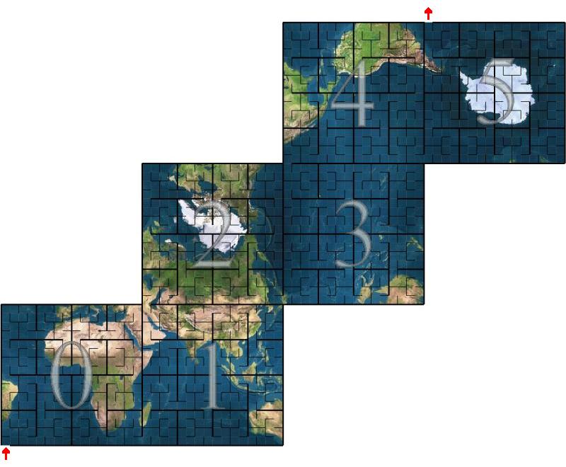
(Larger images of the individual faces can be found here.) Note that the traversal order of the odd-numbered faces is the mirror image of the even-numbered faces.
When the cube is mapped onto the unit sphere, the result is the curve shown earlier:
S2CellId Numbering (again)
We now return to the question of how the S2 cells are numbered. Recall that there are 31 levels of subdivision, ranging from 0 to 30. It turns out that the cell numbering system at all levels follows a very simple rule, namely:
The S2CellId of cell C is the S2 curve parameter at the center of C (scaled to obtain an integer).
For example, consider the level 0 cell for cube face 2. The center of this cell has the S2 curve parameter (in binary):
s = 010.100000000…
where “010” is the binary representation of face 2 and “.1000…” is
the binary representation of 0.5 (i.e., the Hilbert curve parameter at
the center of this face, as discussed above). Scaling this by a factor
of 261, we obtain 0101000… in binary (where there are 60
trailing zeros), or 0x5000000000000000 in hexadecimal. This is the
S2CellId for the level 0 cell on face 2.
It turns out that all S2CellIds up to level 30 can be represented in this
way, i.e. the S2 curve parameters of the corresponding cell centers can be
represented exactly in 64 bits. Note that no two cells (even at different
levels) have the same center position, and therefore all the S2CellIds are
distinct. The cell center is sufficient to specify both the position and
the subdivision level of each cell.
We can also look at this from a more practical point of view. The
S2CellId for a cell at level k always has the following structure:
s = [face] [child]k 1 060-2k
where “face” is a 3-bit number (range 0..5) that selects a cube face, and each of the k “child” values is a 2-bit number that selects one of the 4 children during the subdivision process. The bit that follows the last child is always 1, and all other bits are zero. For example:
010 10000...0         Face cell 2.
001 10 100...0        Subcell 2 of face cell 1.
100 11 01 1000...0    Subcell 1 of subcell 3 of face 4.
This representation has the convenient property that the subdivision level of a cell can easily be determined from the position of its lowest-numbered 1 bit.
Coordinate Systems
The process of mapping an S2CellId to a point on the unit sphere involves
several steps, each with its own coordinate system.
-
(cellid)
Cell id: A 64-bit encoding of a face and a Hilbert curve parameter on that face, as discussed above. The Hilbert curve parameter implicitly encodes both the position of a cell and its subdivision level. -
(face, i, j)
Leaf-cell coordinates: The leaf cells are the subsquares that result after 30 levels of Hilbert curve subdivision, consisting of a 230 × 230 array on each face. “i” and “j” are integers in the range [0, 230-1] that identify a particular leaf cell. The (i, j) coordinate system is right-handed on every face, and the faces are oriented such that Hilbert curves connect continuously from one face to the next. -
(face, s, t)
Cell-space coordinates: “s” and “t” are real numbers in the range [0,1] that identify a point on the given face. For example, the point (s, t) = (0.5, 0.5) corresponds to the center of the cell at level 0. Cells in (s, t)-coordinates are perfectly square and subdivided around their center point, just like the Hilbert curve construction. -
(face, u, v)
Cube-space coordinates: To make the cells at each level more uniform in size after they are projected onto the sphere, we apply a nonlinear transformation of the form u=f(s), v=f(t) before projecting points onto the sphere. This function also scales the (u,v)-coordinates so that each face covers the biunit square [-1,1]×[-1,1]. Cells in (u,v)-coordinates are rectangular, and are not necessarily subdivided around their center point (because of the nonlinear transformation “f”). -
(x, y, z)
Spherical point: The finalS2Pointis obtained by projecting the (face, u, v) coordinates onto the unit sphere. Cells in (x,y,z)-coordinates are quadrilaterals bounded by four spherical geodesic edges.
The purpose of the nonlinear (face, s, t) → (face, u, v) transformation is to make the cells roughly the same size on the sphere. This can be visualized as follows:
 {height=”400”}
This diagram shows a one-dimensional slice of cube face. Starting from the right-hand size, an s- or t-coordinate in the range [0,1] is transformed non-linearly into a u- or v-coordinate in the range [-1,1]. This point is then projected onto the unit sphere.
The purpose of the (face, s, t)→(face, u, v) transformation is illustrated by the two angles marked in red. Although both angles are the same size, and therefore correspond to the same distance on the unit sphere, they have very different sizes when projected back to (u,v)-coordinates (i.e., the top interval on the middle (u,v)-slice is much larger). The non-linear transformation between (s,t) and (u,v) coordinates helps to correct this situation (i.e., the intervals on the right-hand (s,t)-slice are closer in size).
Note that the (i, j), (s, t), and (u, v) coordinate systems are right-handed on all six faces.
S2CellId
The S2CellId class is a thin wrapper over
the 64-bit S2CellId number that provides methods for
navigating the cell hierarchy (finding parents, children, containment tests,
etc). Since leaf cells are often used to represent points on the unit sphere,
the S2CellId class also provides methods for converting directly to and from
an S2Point. Here are its methods:
class S2CellId {
 public:
  static const int kFaceBits = 3;
  static const int kNumFaces = 6;
  static const int kMaxLevel = 30;  // Valid levels: 0..kMaxLevel
  static const int kMaxSize = 1 << kMaxLevel;

  // Although only 60 bits are needed to represent the index of a leaf
  // cell, we need an extra bit in order to represent the position of
  // the center of the leaf cell along the Hilbert curve.
  static const int kPosBits = 2 * kMaxLevel + 1;

  explicit S2CellId(uint64 id);

  // The default constructor returns an invalid cell id.
  S2CellId();
  static S2CellId None();

  // Return an invalid cell id guaranteed to be larger than any
  // valid cell id.  Useful for creating indexes.
  static S2CellId Sentinel();

  // Return the cell corresponding to a given S2 cube face.
  static S2CellId FromFace(int face);

  // Return a cell given its face (range 0..5), Hilbert curve position within
  // that face (an unsigned integer with S2CellId::kPosBits bits), and level
  // (range 0..kMaxLevel).  The given position will be modified to correspond
  // to the Hilbert curve position at the center of the returned cell.  This
  // is a static function rather than a constructor in order to indicate what
  // the arguments represent.
  static S2CellId FromFacePosLevel(int face, uint64 pos, int level);

  // Construct a leaf cell containing the given point "p".  Usually there is
  // exactly one such cell, but for points along the edge of a cell, any
  // adjacent cell may be (deterministically) chosen.  This is because
  // S2CellIds are considered to be closed sets.  The returned cell will
  // always contain the given point, i.e.
  //
  //   S2Cell(S2CellId(p)).Contains(p)
  //
  // is always true.  The point "p" does not need to be normalized.
  explicit S2CellId(const S2Point& p);

  // Construct a leaf cell containing the given normalized S2LatLng.
  explicit S2CellId(const S2LatLng& ll);

  // Return the direction vector corresponding to the center of the given
  // cell.  The vector returned by ToPointRaw is not necessarily unit length.
  // This method returns the same result as S2Cell::GetCenter().
  S2Point ToPoint() const;
  S2Point ToPointRaw() const;

  // Return the S2LatLng corresponding to the center of the given cell.
  S2LatLng ToLatLng() const;

  // The 64-bit unique identifier for this cell.
  uint64 id() const;

  // Return true if id() represents a valid cell.
  bool is_valid() const;

  // Which cube face this cell belongs to, in the range 0..5.
  int face() const;

  // The position of the cell center along the Hilbert curve over this face,
  // in the range 0..(2^kPosBits-1).
  uint64 pos() const;

  // Return the subdivision level of the cell (range 0..kMaxLevel).
  int level() const;

  // Return true if this is a leaf cell (more efficient than checking
  // whether level() == kMaxLevel).
  bool is_leaf() const;

  // Return true if this is a top-level face cell (more efficient than
  // checking whether level() == 0).
  bool is_face() const;

  // Return the child position (0..3) of this cell within its parent.
  // REQUIRES: level() >= 1.
  int child_position() const;

  // Return the child position (0..3) of this cell's ancestor at the given
  // level within its parent.  For example, child_position(1) returns the
  // position of this cell's level-1 ancestor within its top-level face cell.
  // REQUIRES: 1 <= level <= this->level().
  int child_position(int level) const;

  // Methods that return the range of cell ids that are contained
  // within this cell (including itself).  The range is *inclusive*
  // (i.e. test using >= and <=) and the return values of both
  // methods are valid leaf cell ids.
  //
  // These methods should not be used for iteration.  If you want to
  // iterate through all the leaf cells, call child_begin(kMaxLevel) and
  // child_end(kMaxLevel) instead.  Also see maximum_tile(), which can be used
  // to iterate through cell ranges using cells at different levels.
  //
  // It would in fact be error-prone to define a range_end() method, because
  // this method would need to return (range_max().id() + 1) which is not
  // always a valid cell id.  This also means that iterators would need to be
  // tested using "<" rather that the usual "!=".
  S2CellId range_min() const;
  S2CellId range_max() const;

  // Return true if the given cell is contained within this one.
  bool contains(S2CellId other) const;

  // Return true if the given cell intersects this one.
  bool intersects(S2CellId other) const;

  // Return the cell at the previous level or at the given level (which must
  // be less than or equal to the current level).
  S2CellId parent() const;
  S2CellId parent(int level) const;

  // Return the immediate child of this cell at the given traversal order
  // position (in the range 0 to 3).  This cell must not be a leaf cell.
  S2CellId child(int position) const;

  // Iterator-style methods for traversing the immediate children of a cell or
  // all of the children at a given level (greater than or equal to the current
  // level).  Note that the end value is exclusive, just like standard STL
  // iterators, and may not even be a valid cell id.  You should iterate using
  // code like this:
  //
  //   for(S2CellId c = id.child_begin(); c != id.child_end(); c = c.next())
  //     ...
  //
  // The convention for advancing the iterator is "c = c.next()" rather
  // than "++c" to avoid possible confusion with incrementing the
  // underlying 64-bit cell id.
  S2CellId child_begin() const;
  S2CellId child_begin(int level) const;
  S2CellId child_end() const;
  S2CellId child_end(int level) const;

  // Return the next/previous cell at the same level along the Hilbert curve.
  // Works correctly when advancing from one face to the next, but
  // does *not* wrap around from the last face to the first or vice versa.
  S2CellId next() const;
  S2CellId prev() const;

  // This method advances or retreats the indicated number of steps along the
  // Hilbert curve at the current level, and returns the new position.  The
  // position is never advanced past End() or before Begin().
  S2CellId advance(int64 steps) const;

  // Return the level of the "lowest common ancestor" of this cell and
  // "other".  Note that because of the way that cell levels are numbered,
  // this is actually the *highest* level of any shared ancestor.  Return -1
  // if the two cells do not have any common ancestor (i.e., they are from
  // different faces).
  int GetCommonAncestorLevel(S2CellId other) const;

  // Iterator-style methods for traversing all the cells along the Hilbert
  // curve at a given level (across all 6 faces of the cube).  Note that the
  // end value is exclusive (just like standard STL iterators), and is not a
  // valid cell id.
  static S2CellId Begin(int level);
  static S2CellId End(int level);

  // Methods to encode and decode cell ids to compact text strings suitable
  // for display or indexing.  Cells at lower levels (i.e. larger cells) are
  // encoded into fewer characters.  The maximum token length is 16.
  //
  // ToToken() returns a string by value for convenience; the compiler
  // does this without intermediate copying in most cases.
  //
  // These methods guarantee that FromToken(ToToken(x)) == x even when
  // "x" is an invalid cell id.  All tokens are alphanumeric strings.
  // FromToken() returns S2CellId::None() for malformed inputs.
  string ToToken() const;
  static S2CellId FromToken(const char* token, size_t length);
  static S2CellId FromToken(const string& token);

  // Creates a debug human readable string. Used for << and available for direct
  // usage as well.
  string ToString() const;

  // Return the four cells that are adjacent across the cell's four edges.
  // Neighbors are returned in the order defined by S2Cell::GetEdge.  All
  // neighbors are guaranteed to be distinct.
  void GetEdgeNeighbors(S2CellId neighbors[4]) const;

  // Return the neighbors of closest vertex to this cell at the given level,
  // by appending them to "output".  Normally there are four neighbors, but
  // the closest vertex may only have three neighbors if it is one of the 8
  // cube vertices.
  //
  // Requires: level < this->level(), so that we can determine which vertex is
  // closest (in particular, level == kMaxLevel is not allowed).
  void AppendVertexNeighbors(int level, std::vector<S2CellId>* output) const;

  // Append all neighbors of this cell at the given level to "output".  Two
  // cells X and Y are neighbors if their boundaries intersect but their
  // interiors do not.  In particular, two cells that intersect at a single
  // point are neighbors.
  //
  // Requires: nbr_level >= this->level().  Note that for cells adjacent to a
  // face vertex, the same neighbor may be appended more than once.
  void AppendAllNeighbors(int nbr_level, std::vector<S2CellId>* output) const;
};
See s2cellid.h for additional methods.
S2Cell
An S2Cell is an S2Region object that represents a cell. Unlike S2CellId,
it views a cell as a representing a spherical quadrilateral rather than a point,
and it supports efficient containment and intersection tests. However, it is
also a more expensive representation (currently 48 bytes rather than 8).
Here are its methods:
class S2Cell final : public S2Region {
 public:
  // The default constructor is required in order to use freelists.
  // Cells should otherwise always be constructed explicitly.
  S2Cell();

  // An S2Cell always corresponds to a particular S2CellId.  The other
  // constructors are just convenience methods.
  explicit S2Cell(S2CellId id);

  // Convenience constructors.  The S2LatLng must be normalized.
  explicit S2Cell(const S2Point& p);
  explicit S2Cell(const S2LatLng& ll);

  // Return the cell corresponding to the given S2 cube face.
  static S2Cell FromFace(int face);

  // Return a cell given its face (range 0..5), Hilbert curve position within
  // that face (an unsigned integer with S2CellId::kPosBits bits), and level
  // (range 0..kMaxLevel).  The given position will be modified to correspond
  // to the Hilbert curve position at the center of the returned cell.  This
  // is a static function rather than a constructor in order to indicate what
  // the arguments represent.
  static S2Cell FromFacePosLevel(int face, uint64 pos, int level);

  S2CellId id() const;
  int face() const;
  int level() const;
  int orientation() const;
  bool is_leaf() const;

  // Return the k-th vertex of the cell (k = 0,1,2,3).  Vertices are returned
  // in CCW order (lower left, lower right, upper right, upper left in the UV
  // plane).  The points returned by GetVertexRaw are not normalized.
  S2Point GetVertex(int k) const;
  S2Point GetVertexRaw(int k) const;

  // Return the inward-facing normal of the great circle passing through
  // the edge from vertex k to vertex k+1 (mod 4).  The normals returned
  // by GetEdgeRaw are not necessarily unit length.
  S2Point GetEdge(int k) const;
  S2Point GetEdgeRaw(int k) const;

  // If this is not a leaf cell, set children[0..3] to the four children of
  // this cell (in traversal order) and return true.  Otherwise returns false.
  // This method is equivalent to the following:
  //
  // for (pos=0, id=child_begin(); id != child_end(); id = id.next(), ++pos)
  //   children[pos] = S2Cell(id);
  //
  // except that it is more than two times faster.
  bool Subdivide(S2Cell children[4]) const;

  // Return the direction vector corresponding to the center in (s,t)-space of
  // the given cell.  This is the point at which the cell is divided into four
  // subcells; it is not necessarily the centroid of the cell in (u,v)-space
  // or (x,y,z)-space.  The point returned by GetCenterRaw is not necessarily
  // unit length.
  S2Point GetCenter() const;
  S2Point GetCenterRaw() const;

  // Return the average area for cells at the given level.
  static double AverageArea(int level);

  // Return the average area of cells at this level.  This is accurate to
  // within a factor of 1.7 (for S2_QUADRATIC_PROJECTION) and is extremely
  // cheap to compute.
  double AverageArea() const;

  // Return the approximate area of this cell.  This method is accurate to
  // within 3% percent for all cell sizes and accurate to within 0.1% for
  // cells at level 5 or higher (i.e. squares 350km to a side or smaller
  // on the Earth's surface).  It is moderately cheap to compute.
  double ApproxArea() const;

  // Return the area of this cell as accurately as possible.  This method is
  // more expensive but it is accurate to 6 digits of precision even for leaf
  // cells (whose area is approximately 1e-18).
  double ExactArea() const;

  // Return the distance from the cell to the given point.  Returns zero if
  // the point is inside the cell.
  S1ChordAngle GetDistance(const S2Point& target) const;

  // Return the distance from the cell boundary to the given point.
  S1ChordAngle GetBoundaryDistance(const S2Point& target) const;

  // Return the minimum distance from the cell to the given edge AB.  Returns
  // zero if the edge intersects the cell interior.
  S1ChordAngle GetDistance(const S2Point& a, const S2Point& b) const;

  ////////////////////////////////////////////////////////////////////////
  // S2Region interface (see s2region.h for details):

  S2Cell* Clone() const override;
  S2Cap GetCapBound() const override;
  S2LatLngRect GetRectBound() const override;
  bool Contains(const S2Cell& cell) const override;
  bool MayIntersect(const S2Cell& cell) const override;

  // Return true if the cell contains the given point "p".  Note that unlike
  // S2Loop/S2Polygon, S2Cells are considered to be closed sets.  This means
  // that points along an S2Cell edge (or at a vertex) belong to the adjacent
  // cell(s) as well.
  //
  // If instead you want every point to be contained by exactly one S2Cell,
  // you will need to convert the S2Cells to S2Loops (which implement point
  // containment this way).
  //
  // The point "p" does not need to be normalized.
  bool Contains(const S2Point& p) const override;
};
See s2cell.h for additional methods.
S2CellUnion
An S2CellUnion is an S2Region consisting of cells of various sizes. A cell
union is typically used to approximate some other shape. There is a tradeoff
between the accuracy of the approximation and how many cells are used. Unlike
polygons, cells have a fixed hierarchical structure. This makes them more
suitable for spatial indexing.
An S2CellUnion is represented as a vector of sorted, non-overlapping
S2CellIds. By default the vector is also “normalized”, meaning that groups
of 4 child cells have been replaced by their parent cell whenever possible.
S2CellUnions are not required to be normalized, but certain operations will
return different results if they are not (e.g., Contains(S2CellUnion).)
Here is the interface:
class S2CellUnion final : public S2Region {
 public:
  // Creates an empty cell union.
  S2CellUnion() {}

  // Constructs a cell union with the given S2CellIds, then calls Normalize()
  // to sort them, remove duplicates, and merge cells when possible.  (See
  // FromNormalized if your vector is already normalized.)
  //
  // The argument is passed by value, so if you are passing a named variable
  // and have no further use for it, consider using std::move().
  //
  // A cell union containing a single S2CellId may be constructed like this:
  //
  //     S2CellUnion example({cell_id});
  explicit S2CellUnion(std::vector<S2CellId> cell_ids);

  // Convenience constructor that accepts a vector of uint64.  Note that
  // unlike the constructor above, this one makes a copy of "cell_ids".
  explicit S2CellUnion(const std::vector<uint64>& cell_ids);

  // Constructs a cell union from S2CellIds that have already been normalized
  // (typically because they were extracted from another S2CellUnion).
  //
  // The argument is passed by value, so if you are passing a named variable
  // and have no further use for it, consider using std::move().
  //
  // REQUIRES: "cell_ids" satisfies the requirements of IsNormalized().
  static S2CellUnion FromNormalized(std::vector<S2CellId> cell_ids);

  // Constructs a cell union from a vector of sorted, non-overlapping
  // S2CellIds.  Unlike the other constructors, FromVerbatim does not require
  // that groups of 4 child cells have been replaced by their parent cell.  In
  // other words, "cell_ids" must satisfy the requirements of IsValid() but
  // not necessarily IsNormalized().
  //
  // Note that if the cell union is not normalized, certain operations may
  // return different results (e.g., Contains(S2CellUnion)).
  //
  // REQUIRES: "cell_ids" satisfies the requirements of IsValid().
  static S2CellUnion FromVerbatim(std::vector<S2CellId> cell_ids);

  // Constructs a cell union that corresponds to a continuous range of cell
  // ids.  The output is a normalized collection of cell ids that covers the
  // leaf cells between "min_id" and "max_id" inclusive.
  //
  // REQUIRES: min_id.is_leaf(), max_id.is_leaf(), min_id <= max_id.
  static S2CellUnion FromMinMax(S2CellId min_id, S2CellId max_id);

  // Like FromMinMax() except that the union covers the range of leaf cells
  // from "begin" (inclusive) to "end" (exclusive), as with Python ranges or
  // STL iterator ranges.  If (begin == end) the result is empty.
  //
  // REQUIRES: begin.is_leaf(), end.is_leaf(), begin <= end.
  static S2CellUnion FromBeginEnd(S2CellId begin, S2CellId end);

  // Clears the contents of the cell union and minimizes memory usage.
  void Clear();

  // Gives ownership of the vector data to the client without copying, and
  // clears the content of the cell union.  The original data in cell_ids
  // is lost if there was any.
  std::vector<S2CellId> Release();

  // Convenience methods for accessing the individual cell ids.
  int num_cells() const;
  S2CellId cell_id(int i) const;

  // Vector-like methods for accessing the individual cell ids.
  size_t size() const;
  bool empty() const;
  S2CellId operator[](int i) const;

  // Direct access to the underlying vector for STL algorithms.
  const std::vector<S2CellId>& cell_ids() const;

  // Returns true if the cell union is valid, meaning that the S2CellIds are
  // valid, non-overlapping, and sorted in increasing order.
  bool IsValid() const;

  // Returns true if the cell union is normalized, meaning that it is
  // satisfies IsValid() and that no four cells have a common parent.
  // Certain operations such as Contains(S2CellUnion) will return a different
  // result if the cell union is not normalized.
  bool IsNormalized() const;

  // Normalizes the cell union by discarding cells that are contained by other
  // cells, replacing groups of 4 child cells by their parent cell whenever
  // possible, and sorting all the cell ids in increasing order.  Returns true
  // if the number of cells was reduced.
  bool Normalize();

  // Replaces "output" with an expanded version of the cell union where any
  // cells whose level is less than "min_level" or where (level - min_level)
  // is not a multiple of "level_mod" are replaced by their children, until
  // either both of these conditions are satisfied or the maximum level is
  // reached.
  //
  // This method allows a covering generated by S2RegionCoverer using
  // min_level() or level_mod() constraints to be stored as a normalized cell
  // union (which allows various geometric computations to be done) and then
  // converted back to the original list of cell ids that satisfies the
  // desired constraints.
  void Denormalize(int min_level, int level_mod,
                   std::vector<S2CellId>* output) const;

  // If there are more than "excess" elements of the cell_ids() vector that
  // are allocated but unused, reallocate the array to eliminate the excess
  // space.  This reduces memory usage when many cell unions need to be held
  // in memory at once.
  void Pack(int excess = 0);

  // Return true if the cell union contains the given cell id.  Containment is
  // defined with respect to regions, e.g. a cell contains its 4 children.
  // This is a fast operation (logarithmic in the size of the cell union).
  bool Contains(S2CellId id) const;

  // Return true if the cell union intersects the given cell id.
  // This is a fast operation (logarithmic in the size of the cell union).
  bool Intersects(S2CellId id) const;

  // Return true if this cell union contain/intersects the given other cell
  // union.
  bool Contains(const S2CellUnion& y) const;
  bool Intersects(const S2CellUnion& y) const;

  // Returns the union of the two given cell unions.
  S2CellUnion Union(const S2CellUnion& y) const;

  // Returns the intersection of the two given cell unions.
  S2CellUnion Intersection(const S2CellUnion& y) const;

  // Specialized version of GetIntersection() that returns the intersection of
  // a cell union with an S2CellId.  This can be useful for splitting a cell
  // union into pieces.
  S2CellUnion Intersection(S2CellId id) const;

  // Returns the difference of the two given cell unions.
  S2CellUnion Difference(const S2CellUnion& y) const;

  // Expands the cell union by adding a "rim" of cells on expand_level
  // around the union boundary.
  //
  // For each cell c in the union, we add all cells at level
  // expand_level that abut c.  There are typically eight of those
  // (four edge-abutting and four sharing a vertex).  However, if c is
  // finer than expand_level, we add all cells abutting
  // c.parent(expand_level) as well as c.parent(expand_level) itself,
  // as an expand_level cell rarely abuts a smaller cell.
  //
  // Note that the size of the output is exponential in
  // "expand_level".  For example, if expand_level == 20 and the input
  // has a cell at level 10, there will be on the order of 4000
  // adjacent cells in the output.  For most applications the
  // Expand(min_radius, max_level_diff) method below is easier to use.
  void Expand(int expand_level);

  // Expand the cell union such that it contains all points whose distance to
  // the cell union is at most "min_radius", but do not use cells that are
  // more than "max_level_diff" levels higher than the largest cell in the
  // input.  The second parameter controls the tradeoff between accuracy and
  // output size when a large region is being expanded by a small amount
  // (e.g. expanding Canada by 1km).  For example, if max_level_diff == 4 the
  // region will always be expanded by approximately 1/16 the width of its
  // largest cell.  Note that in the worst case, the number of cells in the
  // output can be up to 4 * (1 + 2 ^ max_level_diff) times larger than the
  // number of cells in the input.
  void Expand(S1Angle min_radius, int max_level_diff);

  // The number of leaf cells covered by the union.
  // This will be no more than 6*2^60 for the whole sphere.
  uint64 LeafCellsCovered() const;

  // Approximate this cell union's area by summing the average area of
  // each contained cell's average area, using the AverageArea method
  // from the S2Cell class.
  //
  // NOTE: Since this is proportional to LeafCellsCovered(), it is
  // always better to use the other function if all you care about is
  // the relative average area between objects.
  double AverageBasedArea() const;

  // Calculate this cell union's area by summing the approximate area for each
  // contained cell, using the ApproxArea method from the S2Cell class.
  double ApproxArea() const;

  // Calculate this cell union's area by summing the exact area for each
  // contained cell, using the Exact method from the S2Cell class.
  double ExactArea() const;

  // Return true if two cell unions are identical.
  friend bool operator==(const S2CellUnion& x, const S2CellUnion& y);

  // Return true if two cell unions are different.
  friend bool operator!=(const S2CellUnion& x, const S2CellUnion& y);

  ////////////////////////////////////////////////////////////////////////
  // S2Region interface (see s2region.h for details):

  S2CellUnion* Clone() const override;
  S2Cap GetCapBound() const override;
  S2LatLngRect GetRectBound() const override;
  bool Contains(const S2Cell& cell) const override;
  bool MayIntersect(const S2Cell& cell) const override;

  // The point 'p' does not need to be normalized.
  // This is a fast operation (logarithmic in the size of the cell union).
  bool Contains(const S2Point& p) const override;

  // Appends a serialized representation of the S2CellUnion to "encoder".
  void Encode(Encoder* const encoder) const;

  // Decodes an S2CellUnion encoded with Encode().  Returns true on success.
  bool Decode(Decoder* const decoder);

};
Approximating Regions
An S2RegionCoverer is a class that allows arbitrary regions to be approximated
as unions of cells (S2CellUnion). This is useful for implementing various
sorts of search and precomputation operations.
Typical usage:
S2RegionCoverer::Options options;
options.set_max_cells(5);
S2RegionCoverer coverer(options);
S2Cap cap(center, radius);
S2CellUnion covering = coverer.GetCovering(cap);
The result is a cell union of at most 5 cells that is guaranteed to cover the given cap (a disc-shaped region on the sphere).
The approximation algorithm is not optimal but does a pretty good job in
practice. The output does not always use the maximum number of cells allowed,
both because this would not always yield a better approximation, and because
max_cells() is a limit on how much work is done exploring the possible
covering as well as a limit on the final output size.
The default max_cells() value of 8 is a reasonable point on the
precision/performance tradeoff curve for caps, but you may want to use higher
values for odd-shaped regions, such as long skinny lat-lng rects. Here are some
examples of approximations.
Here is the interface of S2RegionCoverer:
class S2RegionCoverer {
 public:
  class Options {
   public:
    // Sets the desired maximum number of cells in the approximation.  Note
    // that min_level() takes priority over max_cells(), i.e. cells below the
    // given level will never be used even if this causes a large number of
    // cells to be returned.
    //
    // Accuracy is measured by dividing the area of the covering by the area
    // of the original region.  The following table shows the median and worst
    // case values for this area ratio on a test case consisting of 100,000
    // spherical caps of random size (generated using s2regioncoverer_test):
    //
    //   max_cells:        3      4     5     6     8    12    20   100   1000
    //   median ratio:  5.33   3.32  2.73  2.34  1.98  1.66  1.42  1.11   1.01
    //   worst case:  215518  14.41  9.72  5.26  3.91  2.75  1.92  1.20   1.02
    //
    // The default value of 8 gives a reasonable tradeoff between the number
    // of cells used and the accuracy of the approximation.
    //
    // DEFAULT: kDefaultMaxCells
    static constexpr int kDefaultMaxCells = 8;
    int max_cells() const;
    void set_max_cells(int max_cells);

    // Sets the minimum and maximum cell levels to be used.  The default is to
    // use all cell levels.
    //
    // To find the cell level corresponding to a given physical distance, use
    // the S2Cell metrics defined in s2metrics.h.  For example, to find the
    // cell level that corresponds to an average edge length of 10km, use:
    //
    //   int level =
    //       S2::kAvgEdge.GetClosestLevel(S2Earth::KmToRadians(length_km));
    //
    // Note that min_level() takes priority over max_cells(), i.e. cells below
    // the given level will never be used even if this causes a large number
    // of cells to be returned.
    //
    // REQUIRES: max_level() >= min_level()
    // DEFAULT: 0
    int min_level() const;
    void set_min_level(int min_level);

    // DEFAULT: S2CellId::kMaxLevel
    int max_level() const;
    void set_max_level(int max_level);

    // Convenience function that sets both the maximum and minimum cell levels.
    void set_fixed_level(int level);

    // If specified, then only cells where (level - min_level) is a multiple
    // of "level_mod" will be used (default 1).  This effectively allows the
    // branching factor of the S2CellId hierarchy to be increased.  Currently
    // the only parameter values allowed are 1, 2, or 3, corresponding to
    // branching factors of 4, 16, and 64 respectively.
    //
    // DEFAULT: 1
    int level_mod() const;
    void set_level_mod(int level_mod);
  };

  // Constructs an S2RegionCoverer with the given options.
  explicit S2RegionCoverer(const Options& options);

  // Default constructor.  Options can be set using mutable_options().
  S2RegionCoverer();
  ~S2RegionCoverer();

  // Returns the current options.  Options can be modifed between calls.
  const Options& options() const;
  Options* mutable_options();

  // Returns an S2CellUnion that covers (GetCovering) or is contained within
  // (GetInteriorCovering) the given region and satisfies the current options.
  //
  // Note that if options().min_level() > 0 or options().level_mod() > 1, the
  // by definition the S2CellUnion may not be normalized, i.e. there may be
  // groups of four child cells that can be replaced by their parent cell.
  S2CellUnion GetCovering(const S2Region& region);
  S2CellUnion GetInteriorCovering(const S2Region& region);
};
Appendix: Alternatives Considered
The S2 subdivision scheme has a number of advantages over the Hierarchical Triangular Mesh (http://skyserver.org/HTM) framework:
-
Converting from a cell id to a point or vice versa is about 100 times faster than the corresponding HTM operation. For example, a unit vector can be converted to an S2CellId in about 0.15 microseconds, while converting a unit vector to an HTM triangle id takes about 25 microseconds. Similarly, converting an S2CellId to a vector takes about 0.04 microseconds, while the same HTM operation takes about 19 microseconds. (If full resolution is not needed, the HTM times can be improved by using fewer levels – e.g. by using 15 levels rather than 30, conversions are about twice as fast, but the maximum resolution is reduced from 1cm to about 300 meters. The S2 library is still about 100 times faster, though.)
-
The S2 library has no storage requirements. In contrast, the HTM library precomputes the upper levels of the mesh during initialization to get even the performance numbers mentioned above. Computing the first 6 levels (the default) takes about 2MB of memory and 5 milliseconds. It is not practical to precompute much more than this because memory requirements increase by a factor of 4 for each additional level.
-
A linear scan of a set of S2CellIds follows a space-filling curve, which maximizes locality of reference. For example, if each cell id is looked up in a spatial index of some sort, a space-filling curve minimizes the number of times that we switch from one index element to the next. This helps cache performance (including non-local caches such as BigTable). A linear scan through HTM triangles also has fairly good locality of reference due to the hierarchical structure, but it does not define a space-filling curve (due to the triangle ordering chosen by its inventors) and therefore the locality of reference is not as good. (At any given level, the HTM path is about 2.2 times longer than the corresonding S2CellId path.)
Another alternative is HEALPix http://www.eso.org/science/healpix. The main advantage of HEALPix is that it is suitable for calculations involving spherical harmonics. This isn’t relevant to any of our current applications, and the scheme otherwise has several disadvantages from our point of view (e.g. cell boundaries are not geodesics, base structure is more complicated).
The COBE quadrilateralized spherical cube projection (http://lambda.gsfc.nasa.gov/product/cobe/skymap_info_new.cfm) also starts by projecting the six faces of a cube onto the unit sphere, and subdivides each face in a quadtree fashion. However, it does not use a space-filling curve scheme for labelling the cells, the cell edges are not geodesics, and it uses a much more complicated projection scheme designed to minimize distortion.
-
Ideally the converse property would also be true (i.e., if two cells are close together then their
S2CellIdsare also close together), but unfortunately this turns out not to be possible. ↩ -
There are actually 3 different Hilbert curve parameters for the point (0.5, 0.5), corresponding to the fact that the Hilbert curve visits this point 3 times. The three parameters are 0.1000…, 0.00101010…, and 0.11010101… (note that there is another expansion 0.0111… which also visits this point, but it is numerically equal to 0.1000…). This is similar to the fact that there are two decimal expansions of the number 1 (1.000… and 0.999…). In any case, the S2 library only uses the 0.1000… parameter for the cell center. ↩